
Quick links
Definition
Data frame analytics allows you to supercharge your data with extra insights, annotating it using machine learning algorithms. Data frame analytics is an Elasticsearch paid license feature so you will need a paid subscription or a trial license.
Data frame analytic jobs require that the data be organized in tabular format (or data frames). The indices required are entity-centric, which means if you have many records related to the same entity, you must aggregate those into a single document for each entity.
Anomaly detection is a different machine learning technique that is NOT covered in this article.
What are the different types of data frame analytic jobs?
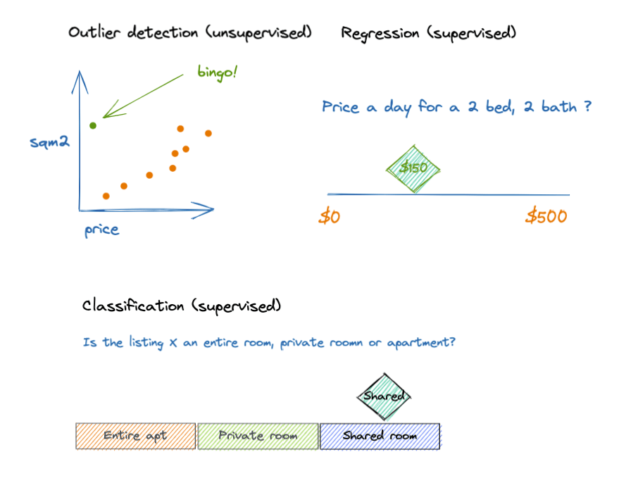
There are three types of data frame analytic jobs:
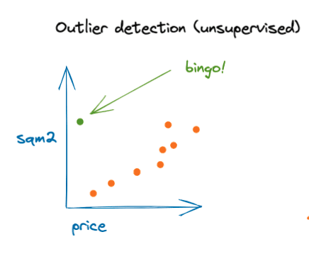
1. Outlier detection (unsupervised): Allows you to detect unusual records based on a set of selected fields (influencers).
2. Regression (supervised): Based on the historical values of a set of fields, you can predict the value of another field.
3. Classification (supervised): Based on a classification field (class), the model can predict the class of new documents according to the values of the companion fields.
Supervised learning requires you to provide data with known values to train the model; unsupervised learning, like anomaly or outlier detection, does not.
Each of the sections below will cover a real-life example of one of the data frame analytics job types.
In the examples that follow, we deal with listings for apartments from Airbnb, and we consider each apartment to be an “entity.” We have one document for each apartment. If that does not apply to your case, you can try using Elasticsearch transform API to achieve your purpose.
1. Outlier detection
In the following example, we will use the Airbnb listings dataset from opendatasoft for New York City.
The goal of this example is to detect unusual listings based on price, number of bedrooms, and number of bathrooms. By doing this, we can detect listing opportunities or capture mistakes made by the owners so we can help them fix the listing posts.
Import sample data
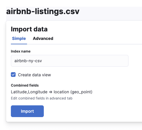
We can easily import the dataset by going to Machine Learning > File in Kibana and loading the CSV file you just exported from opendatasoft:
Keep everything by default, and name the new index airbnb-ny-csv:
This is already an entity-centric dataset (with one document for each apartment listing), so we don’t need any extra transformation and can go ahead and create our outlier detection job.
PRO TIP: After creating the index, we can tune the data view to format the Airbnb links so that they are clickable. Go to Stack Management > Data Views > airbnb-ny-csv > and select the field “Listing Url”, edit and select format as URL.
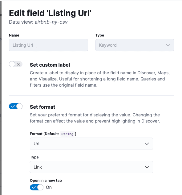
Now, we can click the URLs in Kibana to link to the listing directly. If you want to enrich the data further, you can re-create the data view and select “Host Since” as the timestamp field. That’s optional for this example.
Creating the machine learning job
Now the data is imported, we can go to Analytics > Machine Learning > Create job and select the index we just created.
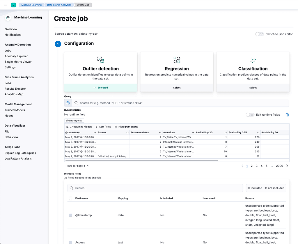
select “Outlier detection,” and you can add a query to filter out some results. If you want to avoid capturing possible mistypes, then adding a price > 10 would be a good idea as it is unlikely that anyone is renting a room or apartment for under $10 in New York. In this example, though, we will keep the box clear.
After that, we must select the fields we want to be analyzed as outlier candidates. In this case, we will select:
* Price
* Bedrooms
* Beds
* Square feet
So, any listing that doesn’t show a “normal” relationship between these fields will have a higher outlier score which will be represented in a new field.
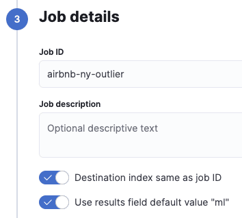
We keep the defaults and then set the job ID to proceed. You can use the same job ID as the destination index or set a different name. Then do the same with the results field. For this example, we will keep both defaults.
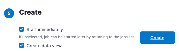
Now, let’s create the job and wait until it finishes:
Visualizing the results
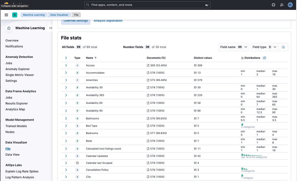
After the job finishes, you can go to “View Results” and select the fields we selected at the beginning. When you do that, you should see something like this:
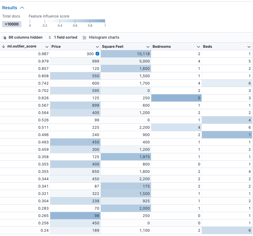
Each of the colored fields contributes to the outlier_score; the darker it is, the more it contributes.
The first result is 10,118 square feet for $300, which looks like a good deal. Note, however, that the exercise is not only about price. For example, although item 7 has the expected relationship between square feet and price, it has no bedrooms.
We can now create a nice dashboard using the results of this exercise:
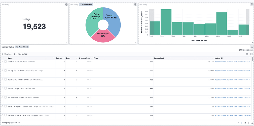
We can see the distribution by room type and the outliers for each host joining year. Now it’s time to explore the data.
Summary of outlier detection
The Elasticsearch data frame analytics feature allows us to very easily detect outliers or “abnormal” results using machine learning algorithms.
The only requirement is to have your data model as “entity-centric,” so if you have the events of your entities over time, you must group those documents and aggregate the fields to obtain the expected results.
2. Regression
Now, let’s look at the second type of data frame analytics job: regression.
We will use the same dataset that we used to test the outlier detection feature. We can do that by following the steps described in the “Import sample data” section above.
Creating the model
When the data is imported, we can go to Analytics > Machine Learning > Create job and select the index we just created:
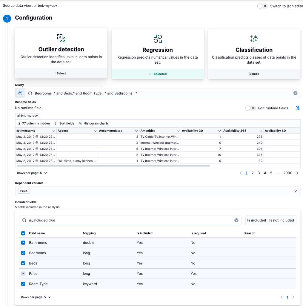
From here, you must select “Regression,” and you can add a query to filter out some results.
For this example, we must filter out the analyzed fields that have empty values for the numeric calculations or the model will fail:
Bedrooms :* and Beds :* and Room Type : * and Bathrooms : *
We set “Price” as the dependent variable because that’s the field we want to predict.
After that, we must select the fields we want to be included in the analysis for the predictions; we will select:
* Bathrooms
* Bedrooms
* Beds
* Room type
It is recommended to keep things simple and select only those fields that you would logically expect to influence the price of the accommodation.

Since this is a supervised learning model, we use part of the data for training and the other part for testing. This way, we can avoid the model being overfitted. A model that’s overfitted will give good results against training data (known values) but perform poorly against uncertain inputs. An 80:20 ratio is a good starting point, so we will keep the defaults:
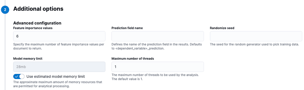
From additional options, we just modify “Feature Importance Values” to 6, which is the total number of fields. Feature importance values help us to interpret the output of our model, showing the impact that each field has on the regression. If a particular feature (analysis field) has a big impact when results are bad, we can remove it from the list to improve our model.
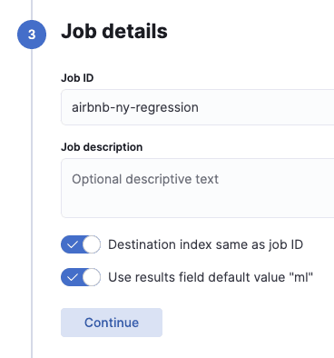
We keep the defaults and then set the job ID to proceed. You can use the same job ID as the destination index or set a different name. Then we do the same with the results field. For this example, we will keep both defaults.
Now, let’s create the job and wait until it finishes:
After it finishes, you can go to “View Results.”
Evaluating the model
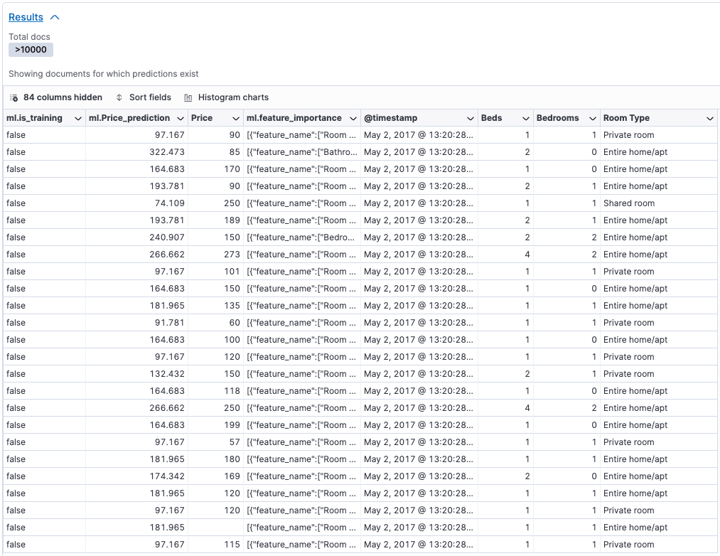
When evaluating the model, the part to look at is at the bottom, in the results section. As you can see, we have a price column and an ml.Price_prediction, which is predicting the value based on the training data.
In this example, some predictions are close; others are not so close. That is because the sample is fairly small (19k records), meaning there is a lot of variance in the results. The more documents you include, and the more distributed the values are, the more precise the predictions will be.
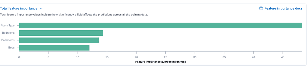
We can also see that the feature with the greatest impact is the room type. That is because it has lower cardinality; so, in small samples, it is a reliable field to include:
See the section below on Recommendations for Supervised Learning for more suggestions on how to improve your models.
Using the model with an inference processor pipeline
Once you have trained the model and decided which fields to use it on and the training period, you can then use the model with the inference ingest pipeline processor.
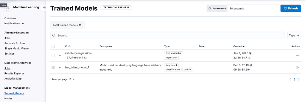
First, go to Machine Learning > Model Management > Trained models and copy the ID of the model you just trained:
Go to Stack Management > Ingest Pipelines and create a new one with the name “airbnb-regression-pipeline”.
Then add a new processor, select the inference processor, and paste the model ID. You should keep the rest of the fields with the defaults:
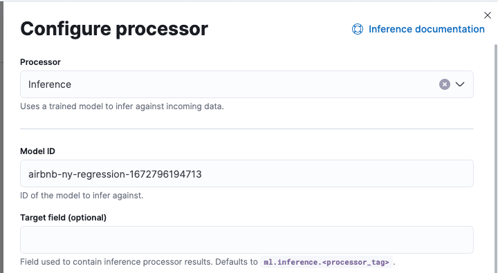
Click Add and then “Create pipeline”.
Now we can go to Management > DevTools, ingest a new listing without price, and use the ingest pipeline to predict the price for us.
First, let’s ingest two listings, an entire apartment and something smaller like a shared room:
POST test_airbnb/_doc?pipeline=airbnb-regression-pipeline
{
  "Beds": 2,
  "Bedrooms": 2,
  "Room Type": "Entire home/apt",
  "Bathrooms": 1
}

POST test_airbnb/_doc?pipeline=airbnb-regression-pipeline
{
  "Beds": 1,
  "Bedrooms": 1,
  "Room Type": "Shared room",
  "Bathrooms": 1
}
Note we applied the ingest pipeline ID as a URL parameter.
Now, let’s run a search to see the results:
GET test_airbnb/_search?_source=ml.inference.Price_prediction,Room Type
That should return something similar to this:
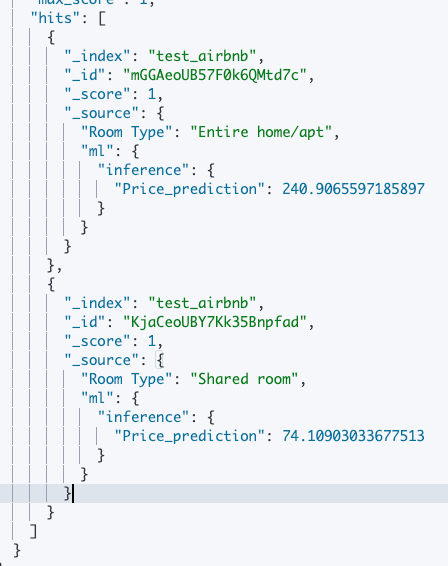
As you can see, privacy is very valuable in New York; the model suggested a much smaller price for the shared room because that’s generally the reality.
Summary of regression
Elasticsearch’s data frame analytics regression feature allows us to train a model with known data and then predict field values for new unknown documents based on this training.
The more data you have, and the more distributed it is, the better. If you have a small sample, you are using too many fields to analyze, or the data is not well distributed, then there is a good chance that your predictions will not be precise. But if you gather enough sufficiently representative data, the results should be very accurate. You can test that by trying with your own data and analysis fields.
3. Classification
In the following example, we will use the same Airbnb listings dataset from opendatasoft that we used in the previous examples.
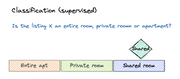
The goal of this example is to predict a category based on some other fields.
In this example, we will train a model to classify listings in:
- Entire house/apartment
- Private room
- Shared room
This is useful to classify listings where we don’t have this information, for example, when they come from another website or database.
This data is already tagged in the RoomType field, so we don’t have to tag it. If you want to generate a field that does not exist in your data, you will have to manually tag a sample of your documents as training data.
After training this model, we can add new data without RoomType, and the room type will be inferred by the model.
The main difference between regression and classification is that regression helps when predicting a quantity, and classification helps when predicting a class or category. There is an overlap when you try to use classification to calculate a numeric type category.
Creating the model
After the data has been imported, we can go to Analytics > Machine Learning > Create job and select the index we just created:
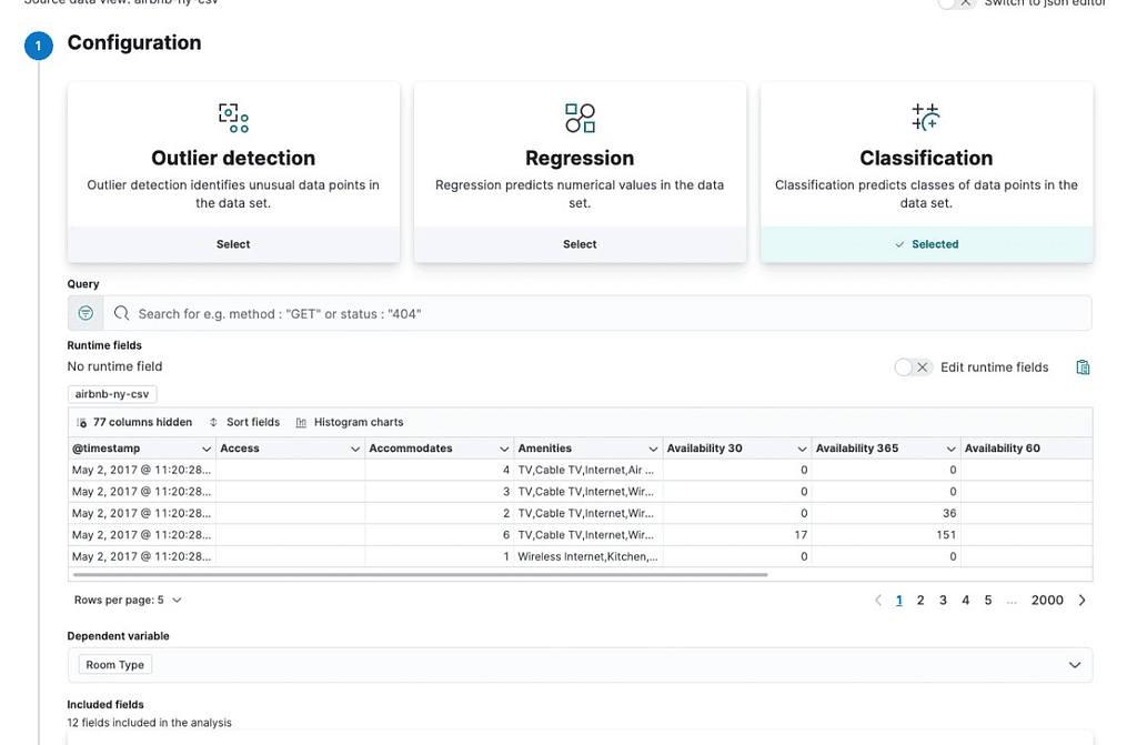
From here you must select “Classification”, and you can add a query to filter out some results. Again, adding a price > 10 could be a good idea if you want to avoid capturing possible mistypes because no one would be renting a room or apartment for less than $10 in NYC. We will keep the box clear.
We set “Room Type” as the dependent variable because that’s the field we want to classify.
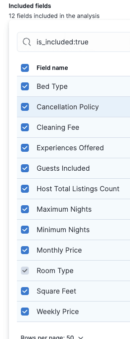
After that, we must select the fields we want to include in the analysis for the classification. We will select all the fields we think are relevant for classifying the room type.

Just as in the regression example, we use part of the data for training and the other part for testing. An 80:20 ratio is a good starting point, so we will keep the defaults:
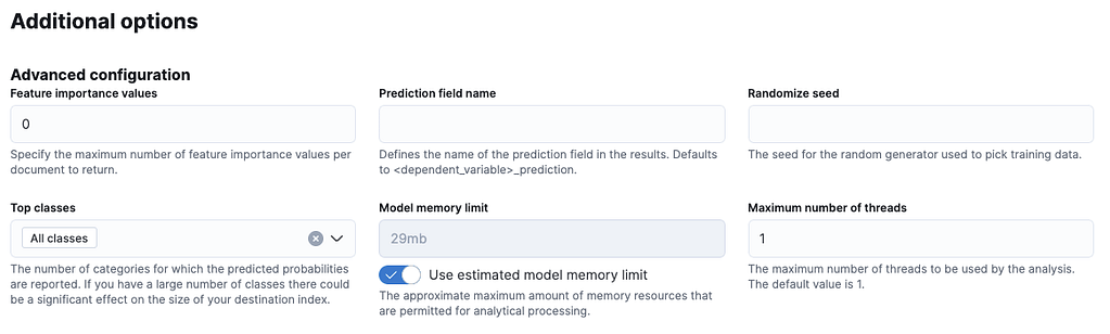
If you have a large number of different classes, you may want to limit the number of classes that are reported. In this example, we only have three classes, so we will select “All classes” here to report all of the probabilities.
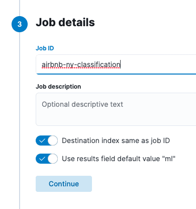
We keep the defaults and then set the job ID to proceed. You can use the same job ID as the destination index or set a different name. The same goes for the results field. For this example, we will keep both defaults.
Now, let’s create the job and wait until it finishes:
After it finishes, you can go to “View Results”.
Evaluating the model
The results page shows us a matrix that gives us a good understanding of the accuracy of our classification:
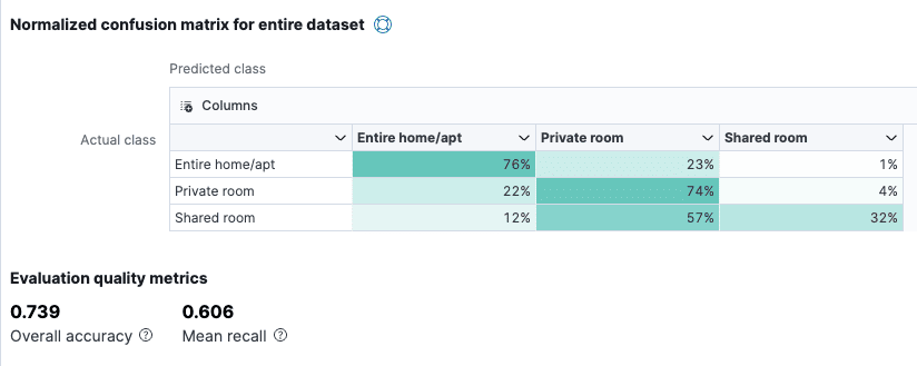
This means that our likelihood of predicting “entire home” correctly was 76% and “private room” 74%. But we were only 32% likely to predict “shared room” correctly.
So, we probably want to do some work to improve the quality of the model, especially in terms of its capability to predict “private rooms.” To do that, we can look at the results section, which will show us the individual score for each of the classifications and the result:
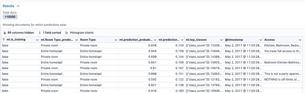
In the second and third columns, you can see the predicted class and the actual class. Prediction_probability and prediction_score (i.e., columns 4 and 5) help us to measure the model confidence. The higher the value, the more confidence.
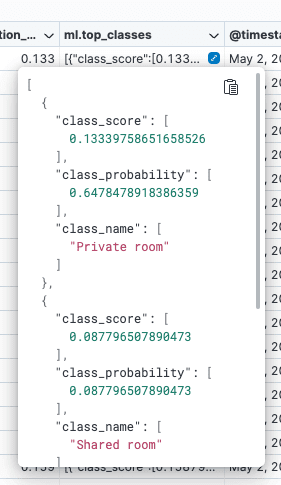
If you expand the top_classes field, you can see the confidence per class:
See the “Recommendations for Supervised Learning” section below for some more suggestions for improving your models.
Using the model with the ingest inference processor
Just as we did with the regression model, we can create an ingest pipeline using the model we have created by using the inference ingest pipeline processor.
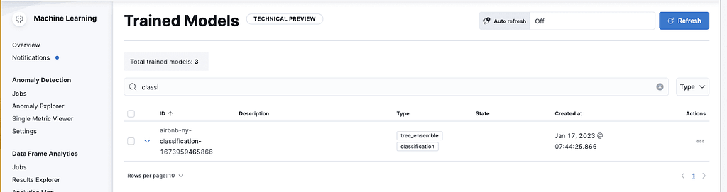
First, go to Machine Learning > Model Management > Trained models and copy the ID of the model you just trained:
Then, go to Stack Management > Ingest Pipelines and create a new one with the name “airbnb-classification-pipeline”.
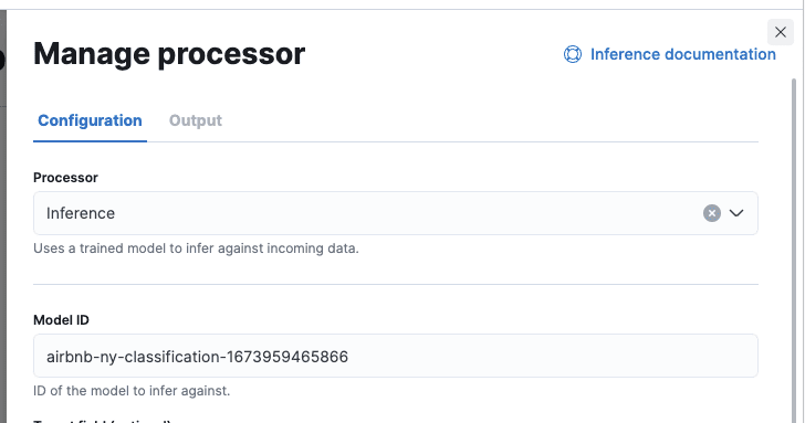
The next step is to add a new processor, select the inference processor, and paste the model ID. We will keep the rest of the fields with the defaults:
Next, click “Add” and then “Create pipeline”.
Now we can go to Management > DevTools, ingest a new listing without “Room Type”, and use the ingest pipeline to predict the class for us.
As an example, let’s ingest one listing with some of the classification fields:
POST test_airbnb/_doc?pipeline=airbnb-classification-pipeline
{
   "Bed Type": "Real Bed",
  "Cancellation Policy": "moderate",
  "Cleaning Fee": 45,
  "Experiences Offered": "none",
  "Guests Included": 1,
  "Host Total Listings Count": 1,
  "Maximum Nights": 500,
  "Minimum Nights": 7,
  "Monthly Price": 8900
}
Note, we applied the ingest pipeline, and not all the classification fields are present.
Now, let’s run a search to see the results:
GET test_airbnb/_search?_source=ml
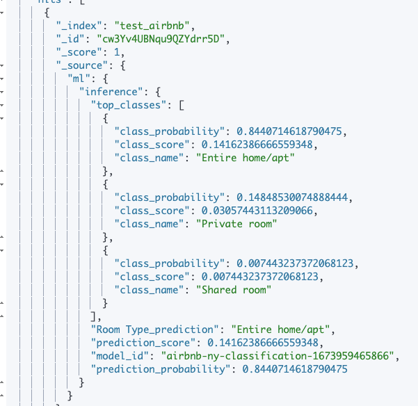
The model predicted the category to be either “entire home” or “apartment” based on the information given.
Now, let’s try it with different values:
POST test_airbnb/_doc?pipeline=airbnb-classification-pipeline
{
   "Bed Type": "Futton",
  "Cancellation Policy": "strict",
  "Cleaning Fee": 25,
  "Experiences Offered": "none",
  "Guests Included": 1,
  "Host Total Listings Count": 1,
  "Maximum Nights": 30,
  "Minimum Nights": 1,
  "Monthly Price": 500
}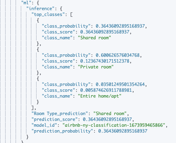
The model now predicts that this apartment is in the shared room category.
Recommendations for supervised learning
These recommendations are appropriate for both regression and classification cases.
Ask yourself the following questions:
- Is the data representative of the population as a whole?
- Is it possible that the training data contains systematic bias?
- Are all of the appropriate influencers included as fields in the data? (For example, property prices can be influenced by the district/neighborhood or the age of the property. Not having this information does not completely invalidate our exercise but will make it harder to predict accurately.)
- Is there a logical reason why the factors you have chosen should affect the outcome? If not, it is probably better to not include them in the model because they only create noise.
- Does each factor have a direct or indirect relationship with what you are trying to predict? For example, price could have a direct relationship with whether or not it is a shared room while the host_total_listings_count (if it has any effect at all) would have a more indirect relationship. In general, it is preferable to use direct relationships with clear causes if they are available, but sometimes we do not have all the data we would like and need to use indirect relationship data as a proxy.
How much training data is required?
While it is generally true to say that more data makes a better model, it is important to reserve part of the data to validate the model. Also, the law of diminishing returns means that we get to a point where extra data does not significantly increase the quality of predictions. Overfitting occurs when we create an overly complex mathematical model that perfectly fits the training data but proves inaccurate as soon as it is tried on new data.
For those reasons, it is important to not use too much training data and to reserve some data for the evaluation of the model. It may be good to start with 20% and slowly increase the percentage to determine whether the quality of the results improves. Once you reach the point where improvement is minimal, then you probably have enough training data.
Summary of classification
Elasticsearch’s data frame analytics classification feature allows us to train a model with known data and then predict a field class (category) for new unknown documents based on that training.
As with the regression feature, the more data you have, and the more distributed it is, the better. If you have a small sample, you are using too many fields to analyze, or the data is not well distributed, then there is a good chance that your predictions will not be precise. But if you gather enough sufficiently representative data, the results should be very accurate. You can test that by trying with your own data and analysis fields.